By
By
What is Classification in Machine Learning?
There are two general types of supervised machine learning approaches in their simplest form. First, you can have a regression problem, where you're trying to predict a continuous variable, such as the temperature or a stock price. The second is a classification problem where you want to predict a categorical variable such as pass/failor spam/ham. Additionally, we can have binary classification problems that we'll cover here with only two outcomes and multi-class classification with more than two outcomes.
Prepping the Data
We want to take several steps to prepare our data for Machine Learning. For text, we want to clean it removing unwanted characters or numbers, we want to remove stop words, or words that appear too frequently, and we also should stem, or lemmatize words, which takes words such as running and runs and brings them to their root form of run. We might want to create new columns or features that aid your machine learning classification process.
For this example, we will use the dataset of Women’s E-Commerce Clothing Reviews on Kaggle.
As always, let's load all the libraries we need to perform this analysis:
# Gereral Imports
import numpy as np
import pandas as pd
import re
import string
from timeit import timeit

# Machine Learning Imports
from sklearn.model_selection import train_test_split
from sklearn.metrics import ConfusionMatrixDisplay
from sklearn.feature_extraction.text import TfidfVectorizer
from sklearn import metrics
from sklearn.model_selection import cross_val_score
from sklearn.model_selection import RepeatedStratifiedKFold
from sklearn.linear_model import LogisticRegression
from sklearn.ensemble import RandomForestClassifier
from sklearn.preprocessing import MinMaxScaler
from sklearn.compose import ColumnTransformer
from sklearn.pipeline import Pipeline

# Model Persistence Imports
from joblib import dump, load

# Test Processing Imports
import nltk
from nltk.stem import PorterStemmer

# Plotting Imports
import matplotlib.pyplot as plt
%matplotlib inline
Feature Engineering
This dataset contains reviews, ratings, department names, and the person's age who wrote the review. The rating system is a classic 1-5 star system. Before cleaning, let's import the data and create a few key columns that we will use in our model, also known as Feature Engineering. We'll use the read_csv function to read the data and create a dataframe called df.
- Since we're performing binary classification, our Target variable needs to be
1or0. In a five-star review system, we can take the4and5star reviews and make them Positive Class and then let the remainder,1,2, and3star reviews be Negative Class. - This particular set of reviews has both a Title and a Review Text field. We can combine these two columns into a new column called Text to simplify our processing.
- As another feature in our model, we can create a new column representing the review text's Total Length.
Note: One step I'm not showing here is EDA or Exploratory Data Analysis. I suggest you always do this before building a model. You can find my process in my post Exploratory Data Analysis.
# Import the data
df = pd.read_csv("ClothingReviews.csv")

# add a column for positive or negative based on the 5 star review
df['Target'] = df['Rating'].apply(lambda c: 0 if c < 4 else 1)

# Combine the title and text into a single column
df['Text'] = df['Title'] + ' ' + df['Review Text']

# Create a new column that is the length of the next text field
df['text_len'] = df.apply(lambda row: len(row['Text']), axis = 1)
Cleaning the Text
Next, we need to clean the text. I've created a function adapted to almost any NLP cleaning situation. Let's take a look at the text before text:
' Love this dress! it\'s sooo pretty. i happened to find it in a store, and i\'m glad i did bc i never would have ordered it online bc it\'s petite. i bought a petite and am 5\'8". i love the length on me- hits just a little below the knee. would definitely be a true midi on someone who is truly petite.'
def process_string(text):

    final_string = ""

    # Convert the text to lowercase
    text = text.lower()

    # Remove punctionation
    translator = str.maketrans('', '', string.punctuation)
    text = text.translate(translator)

    # Remove stop words and usless words
    text = text.split()
    useless_words = nltk.corpus.stopwords.words("english")
    text_filtered = [word for word in text if not word in useless_words]

    # Remove numbers
    text_filtered = [re.sub('\w*\d\w*', '', w) for w in text_filtered]

    # Stem the text with NLTK PorterStemmer
    stemmer = PorterStemmer()
    text_stemmed = [stemmer.stem(y) for y in text_filtered]

    # Join the words back into a string
    final_string = ' '.join(text_stemmed)

    return final_string
We use the Pandas apply method to run this on our Data Frame. After applying this function, let's look at the resulting string.
df['Text_Processed'] = df['Text'].apply(lambda x: process_string(x))
'love dress sooo pretti happen find store im glad bc never would order onlin bc petit bought petit love length hit littl knee would definit true midi someon truli petit'
We can see that the string is perfectly clean, free of numbers, punctuation, stop words, and the words are stemmed into their most simple forms. We're almost ready to start building our model!
Testing for Imbalanced Data
We must understand if our dataset is imbalanced between the two classes in our Target. We can do this quickly with one line of code from Pandas. Imbalanced data is where one class has far more observations than the other. When we train our model, the result will be that the model will be biased towards the class with the most observations.
df['Target'].value_counts()
1    17433
0     5193
Name: Target, dtype: int64
The counts let us know that the data is imbalanced. There is three times the number of positive class 1 observations versus the negative class 0. We will have to make sure that we handle the imbalance appropriately in our model. I'll cover a couple of different ways in this article.
Pipeline Building
Pipelines are a must in properly building a Machine Learning model. They help you organize all the steps it takes to transform data and use your model repeatedly. You can do these steps individually, but when applying your model to new data, it won't be easy if you do not do it this way. Later, I'll show you how this works in practice on new data, but let's build the Pipeline for now.
We have a function for creating a Pipeline. The Pipeline is wrapped in a function to leverage for more than one model as we evaluate our options.
First in the function is a Column Transformer. A column transformer allows us to preprocess data in any number of ways that are appropriate for our model. There are many different ways to transform your data, and I'll not cover them all here, but let me explain the two we're using.
- TfidfVectorizer: the TF-IDF vectorizer transforms text into numeric values. For a great description of this, check out my post on BoW and TF-IDF. Here we're transforming our
Text_Processedcolumn. - MinMaxScaler: This transforms all numeric values into a range between
0and1. Most ML algorithms do not handle data with a wide range of values; it's always a best practice to scale your data. You can read more about this on Scikit-Learn's documentation. Here we're scaling ourtext_lencolumn.
Second is the creation of the Pipeline itself. The Pipeline lists the steps we want to run on the data. We have a fairly simple Pipeline here, but you can add as many steps as you'd like. We have the following.
- prep: This is the column transformer from above. It's going to vectorize our text and scale our text length.
- clf: This is where we choose an instance of our classifier. You can see that this is passed into our function, and we pass it into the function to test different classifiers with the same data.
Note: An instance of a classifier is simply the class itself. For example, LogisticRegression() is an instance of LogisticRegression.
def create_pipe(clf):

    column_trans = ColumnTransformer(
            [('Text', TfidfVectorizer(), 'Text_Processed'),
             ('Text Length', MinMaxScaler(), ['text_len'])],
            remainder='drop')

    pipeline = Pipeline([('prep',column_trans),
                         ('clf', clf)])

    return pipeline
Model Selection via Cross-Validation
When building a machine learning model, a best practice is to perform as Model Selection. Model Selection lets you test different algorithms on your data and determine which performs best. First, we will split our dataset into X and y datasets. X represents all of the features of our model, and y will represent the target variable. The target is the variable we're trying to predict.
X = df[['Text_Processed', 'text_len']]
y = df['Target']
Now it's time to Cross Validate two classifiers. Cross-validation is the process of partitioning data into n number of different splits, which you then use to validate your model. Cross-Validation is important because, in some cases, the observations it learns from in the train set might not represent the observations in the test set. Therefore, you avoid this by running through different data slices. Read more about this on Scikit-Learn's documentation.
Important: One thing I want to bring special attention to below is RepeatedStratifiedKFoldfor cross-validation. A Stratified cross validator will ensure in the case of imbalanced data that the partitions preserve relative class frequencies in the split.
Finally, we will use a classifier that supports the class_weight parameter dealing with imbalanced data. A handful of models from Scikit-Learn support this, and simply by setting the value to balanced, we can account for imbalanced data. Other methods include SMOTE (synthetic generation of minority class observations to balance the data, but this is a great place to start. You can read more about working with imbalanced datafrom my other post.
models = {'LogReg' : LogisticRegression(random_state=42,
                                        class_weight='balanced',
                                        max_iter=500),
          'RandomForest' : RandomForestClassifier(
                                        class_weight='balanced',
                                        random_state=42)}

for name, model, in models.items():
    clf = model
    pipeline = create_pipe(clf)
    cv = RepeatedStratifiedKFold(n_splits=10,
                                 n_repeats=3,
                                 random_state=1)
    %time scores = cross_val_score(pipeline, X, y,
                             scoring='f1_weighted', cv=cv,
                             n_jobs=-1, error_score='raise')
    print(name, ': Mean f1 Weighted: %.3f and StdDev: (%.3f)' % \
        (np.mean(scores), np.std(scores)))
CPU times: user 23.2 s, sys: 10.7 s, total: 33.9 s
Wall time: 15.5 s
LogReg : Mean f1 Weighted: 0.878 and StdDev: (0.005)
CPU times: user 3min, sys: 2.35 s, total: 3min 2s
Wall time: 3min 2s
RandomForest : Mean f1 Weighted: 0.824 and StdDev: (0.008)
In the above function, you can see that scoring is done with f1_weighted. Choosing the right metric is a whole discussion that is critical to understand. I've written about how to choose the right evaluation metric.
Here is a quick explanation of why I chose this metric. First, we have Imbalanced data, and we never want to use accuracy as our metric. Accuracy on imbalanced data will give you a false sense of success, but accuracy will bias the class with more observations. There is also precision and recall which will help you minimize false positives (precision) or minimize false negatives (recall). Depending on the outcomes you want to optimize for, you might choose one of these.
Since we don't prefer to predict positive reviews versus negative reviews, in this case, I've chosen the F1 score. F1 by definition, is the harmonic mean of Precision and Recall combining them into a single metric. However, there is also a way to tell this metric to score imbalanced data with the weighted flag. As the Sciki-learn documentation states:
Calculate metrics for each label and find their average weighted by support (the number of true instances for each label). This alters ‘macro’ to account for label imbalance; it can result in an F-score between precision and recall.
Based on these results, we can see that the LogisticRegression classifier performs slightly better and is much faster, 15 seconds versus 3 minutes. Therefore we can move forward and train our model with it.
Again, please read my full explanation of Model Evaluation to give you a better sense of which one to use and when.
Model Training and Validation
We're finally here! It's time to train our final model and validate it. We'll split our data into training and test partitions since we didn't do this when we performed Cross-Validationabove. You never want to train your model on all of your data, but rather leave a portion out for testing. Whenever a model has seen all data during training, it will know the data and cause overfitting. Overfitting is a problem where a model is too good at predicting the data it has seen and is not generalizable to new data.
# Make training and test sets
X_train, X_test, y_train, y_test = train_test_split(X,
                                                    y,
                                                    test_size=0.33,
                                                    random_state=53)
Next, a quick function will fit our model and evaluate it with a classification_reportand a Confusion Matrix (CM). I believe it's critical to run the classification report along with the CM, and it will show you each of your key evaluation metrics and tell you how the model performed. The CM is a great way to visualize the results.
def fit_and_print(pipeline, name):

    pipeline.fit(X_train, y_train)
    y_pred = pipeline.predict(X_test)

    print(metrics.classification_report(y_test, y_pred, digits=3))

    ConfusionMatrixDisplay.from_predictions(y_test,
                                            y_pred,
                                            cmap=plt.cm.YlOrBr)

    plt.tight_layout()
    plt.ylabel('True label')
    plt.xlabel('predicted label')
    plt.tight_layout()
    plt.savefig('classification_1.png', dpi=300)
clf = LogisticRegression(random_state=42,
                         class_weight='balanced',
                         max_iter=500)
pipeline = create_pipe(clf)
fit_and_print(pipeline, 'Logistic Regression')
              precision    recall  f1-score   support

           0      0.681     0.855     0.758      1715
           1      0.953     0.881     0.915      5752

    accuracy                          0.875      7467
   macro avg      0.817     0.868     0.837      7467
weighted avg      0.891     0.875     0.879      7467
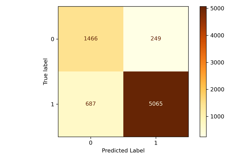
The results are in! The classification report shows us everything we need. Because we said we don't necessarily want to optimize for the positive or negative class, we will use the f1-score column. We can see the 0 class performed at 0.758 and the 1 class at 0.915. You can expect the larger class to perform better whenever you have imbalanced data, but you can use some of the above steps to increase the model's performance.
92% of the time, the model will correctly classify reviews for the positive class and 76% of the time for the negative class. That's quite impressive by simply looking at the text a user has submitted for a review!
Persisting the Model
We can easily persist our model for later use. Because we used a pipeline to build the model, we performed all of the necessary steps to preprocess our data and run the model. Persisting the model makes it easy to run it on a production server or load later and not train it again. After it's saved to disk, it's incredible that this model is less than 500KB on disk!
# Save the model to disk
dump(pipeline, 'binary.joblib')

# Load the model from disk when you're ready to continue
pipeline = load('binary.joblib')
Testing on New Data
Now for a demonstration of what's truly the important part. How well does your model predict new observations it has never seen before? This process would be very different in production, but we can simulate it by creating a few new reviews for a quick example. I've also created a function that transforms a list of strings into the properly formatted data frame with cleaned text and the text_len column.
def create_test_data(x):

    x = process_string(x)
    length = len(x)

    d = {'Text_Processed' : x,
        'text_len' : length}

    df = pd.DataFrame(d, index=[0])

    return df
revs = ['This dress is gorgeous and I love it and would gladly reccomend it.',
        'This skirt has really horible quality and I hate it!',
        'A super cute top with the perfect fit.',
        'The most gorgeous pair of jeans I have seen.',
        'this item is too little and tight.']
print('Returns 1 for Positive reviews and 0 for Negative reviews:','\n')
for rev in revs:
    c_res = pipeline.predict(create_test_data(rev))
    print(rev, '=', c_res)
Returns 1 for Positive reviews and 0 for Negative reviews:

This dress is gorgeous and I love it and would gladly reccomend. = [1]
This skirt has really horible quality and I hate it! = [0]
A super cute top with the perfect fit. = [1]
The most gorgeous pair of jeans I have seen. = [1]
this item is too little and tight. = [0]
Conclusion
There you have it! An end-to-end example of building a binary classifier. It can be simple to build one in a few steps, but this post outlines the preferred steps you should use to properly build your classifier. We started with cleaning the data and some lightweight Feature Engineering, Pipeline building, Model Selection, Model Training and Evaluation, and finally, Persisting the Model. We finished by testing it on new data as well. This workflow should apply to almost any binary or multi-class classification problem. Enjoy and happy model building!
There are two other steps I left out of here, which I'll cover at a later time. Feature Selection and Hyperparameter Tuning. Depending on the complexity of your data, you will want to dig into Feature Selection and to squeeze out the most performance of your model, check out Hyperparameter Tuning.
All of the code for this post is available here in GitHub